Preparations for Next Moonwalk Simulations Underway (and Underwater)
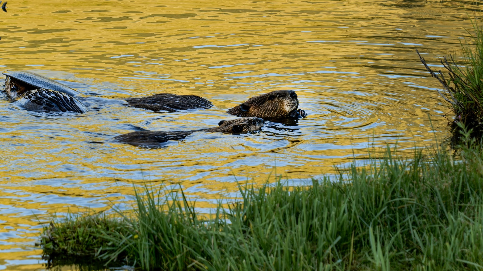
A beaver family nibbles on aspen branches just up Logan Canyon from Utah State University, in Spawn Creek, Utah.
Credit: Sarah Koenigsberg
Humans aren't the only mammals working to mitigate the effects of climate change in the Western United States. People there are also enlisting the aid of nature's most prolific engineers - beavers. Using NASA-provided grants, two open-source programs from Boise State University in Idaho and Utah State University in Logan are making it possible for ranchers, land trust managers, nonprofits, and others to attract beavers to areas that need their help.
The Beaver Restoration Assessment Tool (BRAT) created by Utah State University uses data from satellites built at NASA's Goddard Space Flight Center in Greenbelt, Maryland, to identify areas that need restoration and would benefit from beavers' dam-building abilities. The Boise State University Mesic Resource Restoration Monitoring Aid (MRRMaid) program, which also uses satellite data, monitors the areas over time. Both efforts are also supported by
NASA's Research Opportunities in Space and Earth Science
program and the agency's Applied Sciences'
Ecological Conservation
program.
Once a site is chosen, program staffers and landowners begin to take measures to attract beavers, or the teams may relocate them from other areas. Either way, once on site, these semiaquatic builders get to work building and maintaining dams to create the ponds. The ponds help to retain water, including runoff from snowmelt and rainstorms, that would otherwise rush through the area, causing erosion and degrading the surrounding ecosystems.
Over time, these new ponds raise the water table, support wetlands that attract more wildlife and fish, and restore native plants to the ecosystem. Beaver dams can help ranchers improve water availability on their property, supporting their operations.
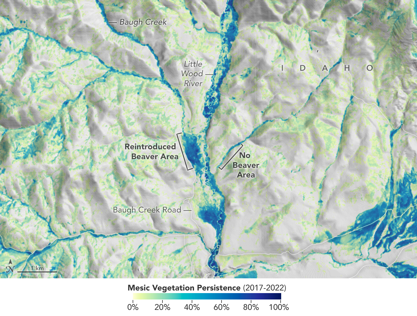
NASA Landsat data helps Utah State University identify streams where beavers can be reintroduced to help improve an ecosystem. Boise State University also uses Landsat data to show just how much beavers help. The vegetation in this satellite image indicates where streams or creeks are flowing and reveals the benefits of beaver activity.
Credit: NASA
In addition to being beautiful and supporting the local ecology, these moisture-rich environments can limit wildfire damage with a barrier of healthy vegetation resistant to burning. When human infrastructure is nearby, a built-in leak or other interventions by humans can be added to control the water level, preventing floods that cause property damage.
As a restoration site's health improves, MRRMaid and BRAT use NASA satellite data to monitor those changes and analyze how the beavers benefit the ecosystem in drought-stricken areas. Community leaders can use this information and the living examples of restored sites to build new parks and recreational areas and plan future restoration projects with their furry collaborators.
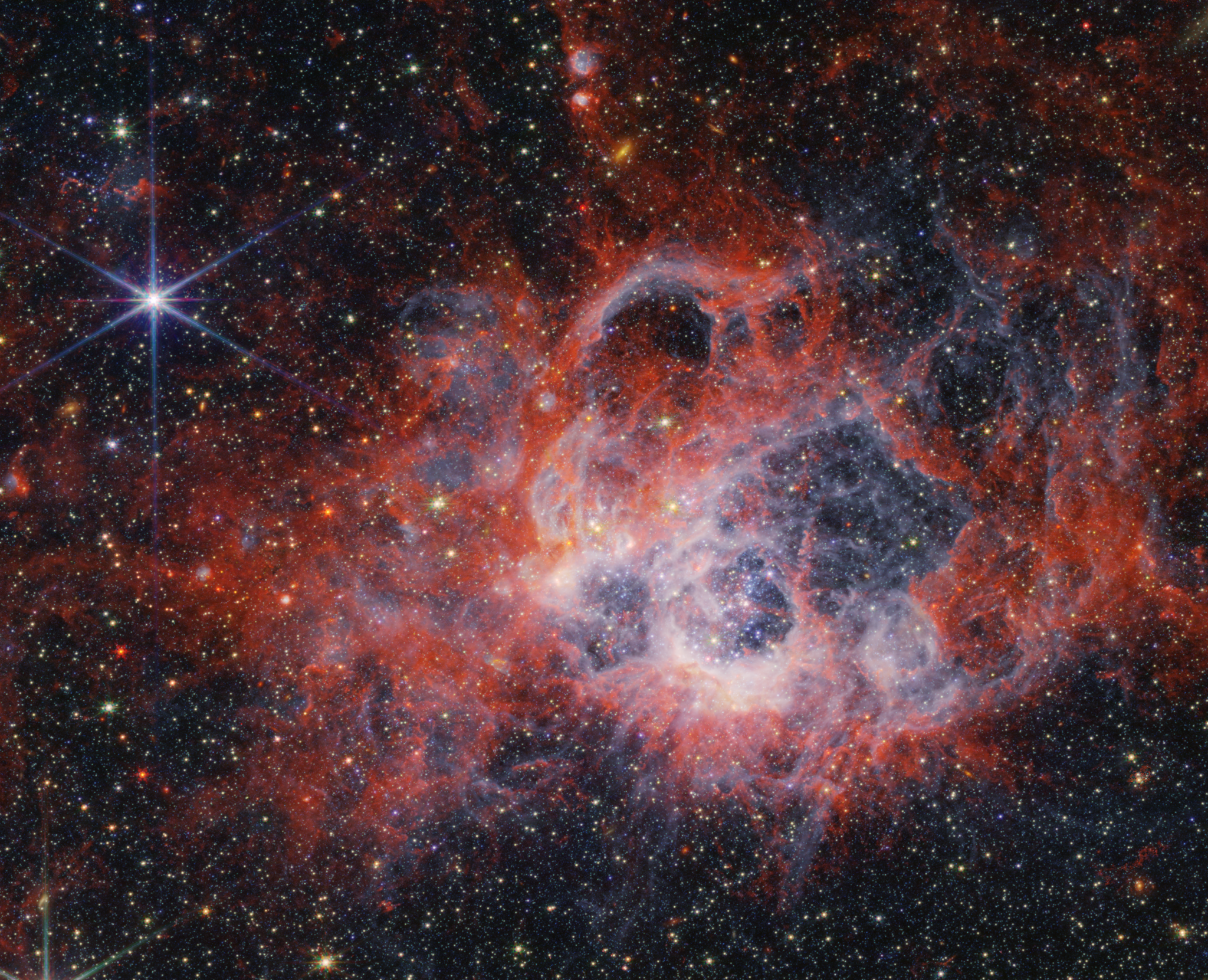
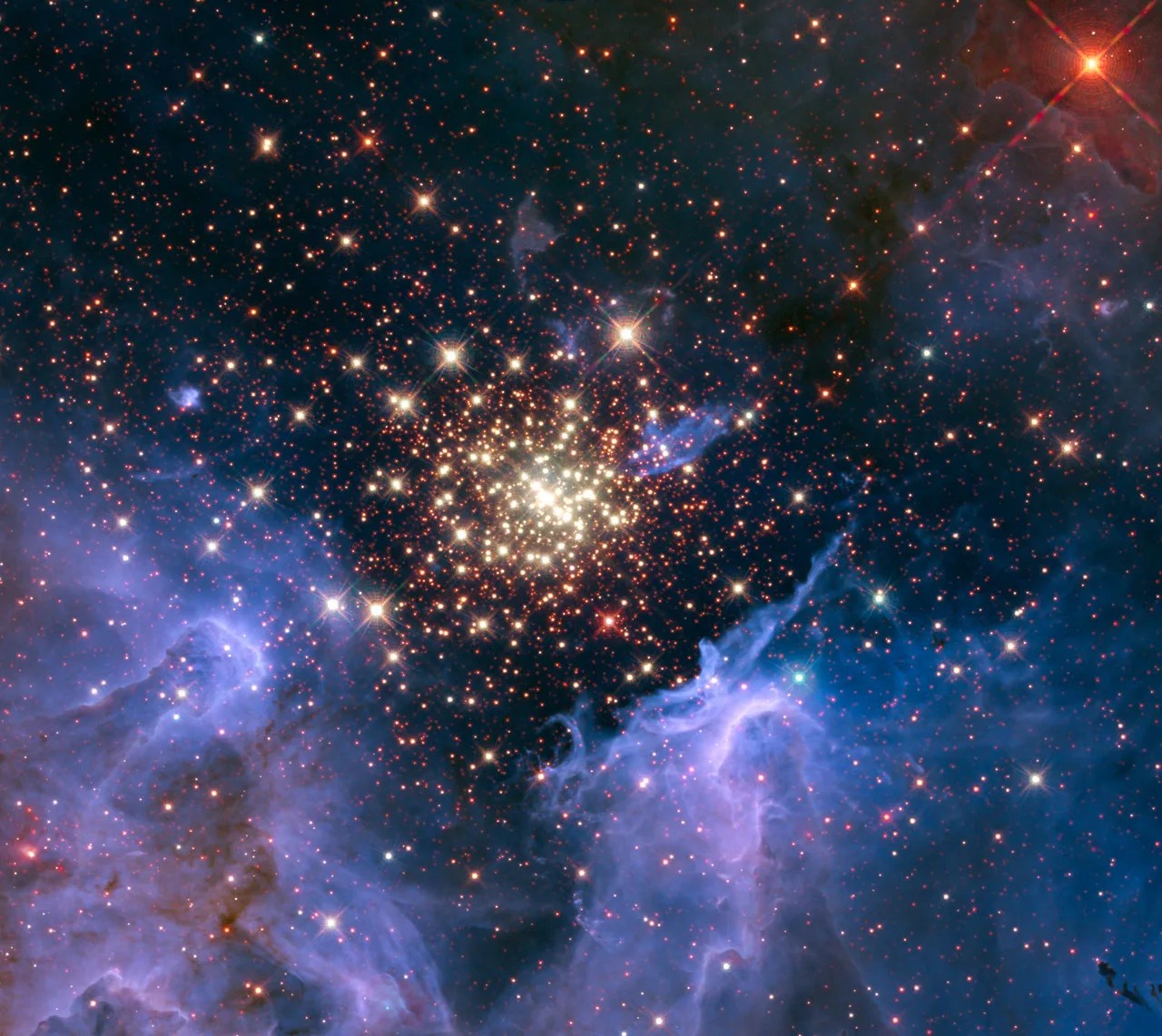
This image from NASA's James Webb Space Telescope's NIRCam (Near-Infrared Camera) of star-forming region NGC 604 shows how stellar winds from bright, hot young stars carve out cavities in surrounding gas and dust.
NASA, ESA, CSA, STScI
In this image released on March 9, 2024, the NIRCam (Near-Infrared Camera) on NASA's James Webb Space Telescope gives us a more detailed view of a well-studied but still mysterious region, NGC 604. The most noticeable features are tendrils and clumps of emission that appear bright red, extending out from areas that look like clearings, or large bubbles in the nebula. Stellar winds from the brightest and hottest young stars have carved out these cavities, while ultraviolet radiation ionizes the surrounding gas. This ionized hydrogen appears as a white and blue ghostly glow.
Learn more about this image and another of the same region from Webb's MIRI (Mid-Infrared Instrument).
Image Credit: NASA, ESA, CSA, STScI
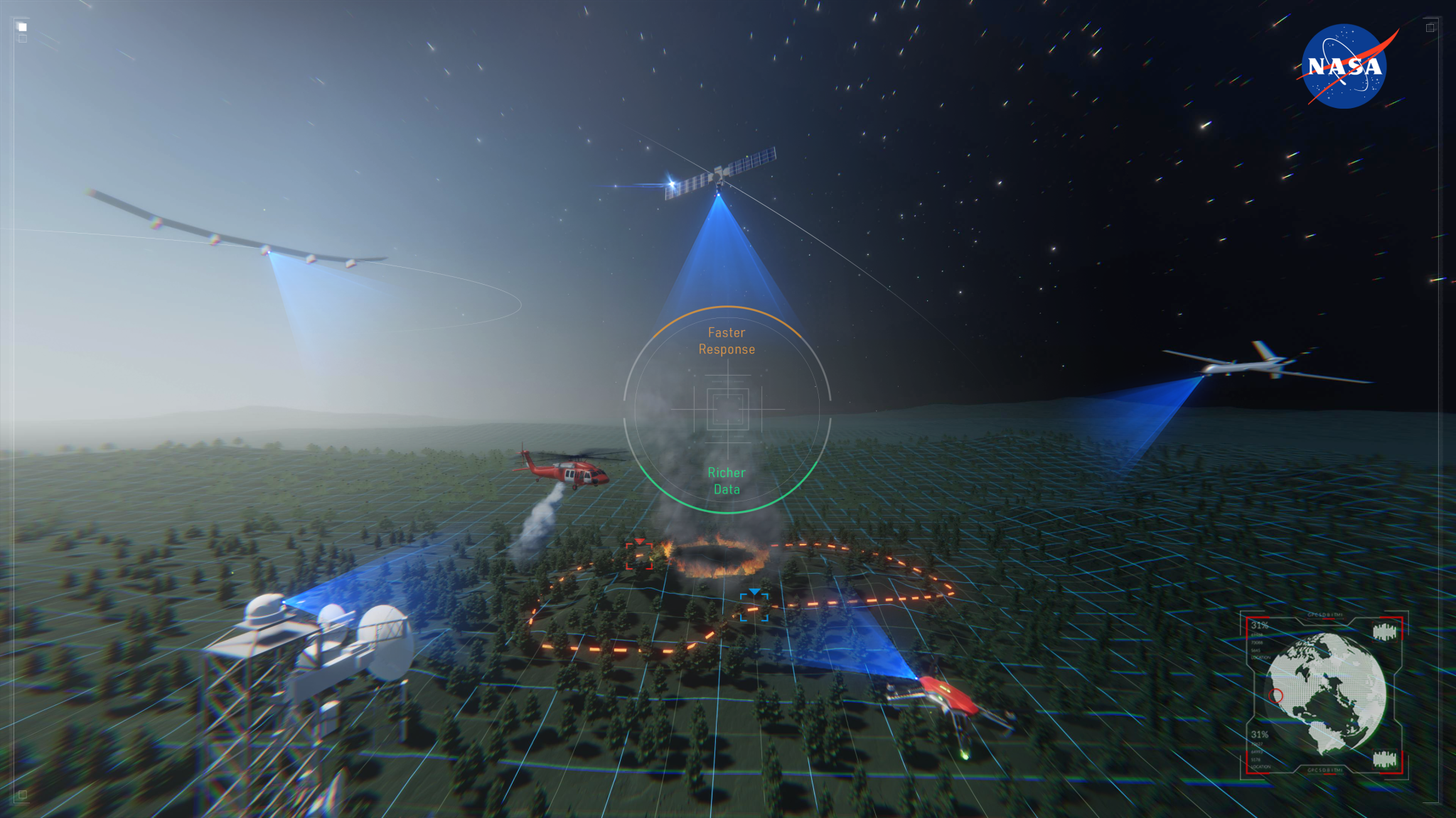
Artist's rendering of remotely piloted aircraft providing fire suppression, monitoring and communications capabilities during a wildland fire.
NASA
NASA and the Federal Aviation Administration (FAA) have established a research transition team to guide the development of wildland fire technology.
Wildland fires are occurring more frequently and at a larger scale than in past decades, according to the U.S. Forest Service. Emergency responders will need a broader set of technologies to prevent, monitor, and fight these growing fires more effectively. Under this Wildland Fire Airspace Operations research transition team, NASA and the FAA will develop concepts and test new technologies to improve airspace integration.
Current aerial firefighting operations are limited to times when aircraft have clear visibility - otherwise pilots run the risk of flying into terrain or colliding with other aircraft. Drones could overcome this limitation by enabling responders to remotely monitor and suppress these fires during nighttime and low visibility conditions, such as periods of heavy smoke. However, advanced airspace management technologies are needed to enable these uncrewed aircraft to stay safely separated and allow aircraft operators to maintain situational awareness during wildland fire management response operations.
Over the next four years, NASA's Advanced Capabilities for Emergency Response Operations (
ACERO
) project, in collaboration with the FAA, will work to develop new airspace access and traffic management concepts and technologies to support wildland fire operations. These advancements will help inform a concept of operations for the future of wildland fire management under development by NASA and other government agencies. The team will test and validate uncrewed aircraft technologies for use by commercial industry and government agencies, paving the way for integrating them into future wildland fire operations.
ACERO is led out of NASA's Ames Research Center in Silicon Valley under the agency's Aeronautics Research Mission Directorate.
NASA invites you - and everyone else on the planet - to take part in a worldwide celebration of Earth Day with the agency’s #GlobalSelfie event. While NASA satellites constantly look at Earth from space, on Earth Day we’re asking you to step outside and take a picture of yourself in your corner of the world. Then post it to social media using the hashtag #GlobalSelfie.
Bonus points if your #GlobalSelfie features your favorite body of water! About 71% of our Blue Marble is covered by water, and that water is one of the main reasons why Earth is like no other planet we've found in this solar system, or beyond.
Why #GlobalSelfie?
NASA astronauts brought home the first ever images of the whole planet from space. Now NASA satellites capture new images of Earth every second. With Earth-observing missions orbiting our home planet right now, and more set to launch this year, NASA studies Earth’s atmosphere, land and oceans in all their complexity.
For Earth Day, we want everyone to share the planet from their point of view. Need an idea of what kind of picture to take? Get outside and show us mountains, parks, the sky, rivers, lakes - and you! Wherever you are, there’s your picture.
How do I take part?
Post your photo to social media using the hashtag #GlobalSelfie. Make it public so we can see, and celebrate #EarthDay with you!
NASA Selects New Aircraft-Driven Studies of Earth and Climate Change
NASA has selected six new airborne missions that include domestic and international studies of fire-induced clouds, Arctic coastal change, air quality, landslide hazards, shrinking glaciers, and emissions from agricultural lands. NASA's suite of airborne missions complement what scientists can see from orbit, measure from the ground, and simulate in computer models.
Funded through the agency's Earth Venture program, the missions center around the use of instruments mounted on aircraft to make measurements in finer detail-both in spatial resolution and shorter time scales-than can be made by many satellites. Competitively selected, the missions provide opportunities to supplement satellite observations and make innovative measurements.
"These missions will help us interpret what our current satellites are seeing from space and test new ideas and techniques for our upcoming Earth System Observatory," said Karen St. Germain, director of NASA's Earth Science Division. "There is also a strong focus on actionable Earth science-gathering fundamental observations that have connections to our economy and societal decision-making and information needs."
NASA's newest Earth Ventures missions include studies of how climate change is altering carbon emissions and water and ice flows across Arctic coastal regions.
Credit: Landsat/USGS/NASA Earth Observatory
Roughly $120 million has been allotted for the six missions, which will deploy at various times from 2026 to 2029. Three lead investigators were chosen for each mission, with at least one required to be an early career scientist. Full staffing of the science teams and selection of complementary instruments will be competed in the coming months. These changes in the selection process were made to promote diversity, equity, and inclusion in the teams.
"We are constantly looking to foster the growth of the next generation of scientists," said Barry Lefer, the program manager who led the Earth Venture selection panels at NASA Headquarters in Washington. "This round of missions will put an extra emphasis on bringing new people into mission planning and leadership."
The six missions include:
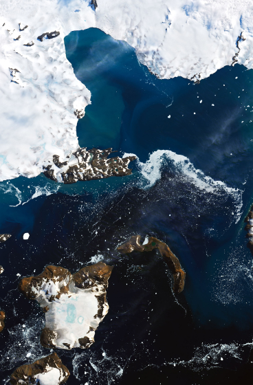
Arctic coastal change
Maria Tzortziou of the City College of New York will lead a project to observe changes in river systems on the North Slope of Alaska. Known as FORTE (short for Arctic Coastlines-The Frontlines of Rapidly Transforming Ecosystems), the project will combine optical and radar measurements from planes, helicopters, boats, and drones to measure water flows and chemistry and observe how ecosystems respond to changing climate. The team will collaborate with indigenous communities to sustain observations over time.
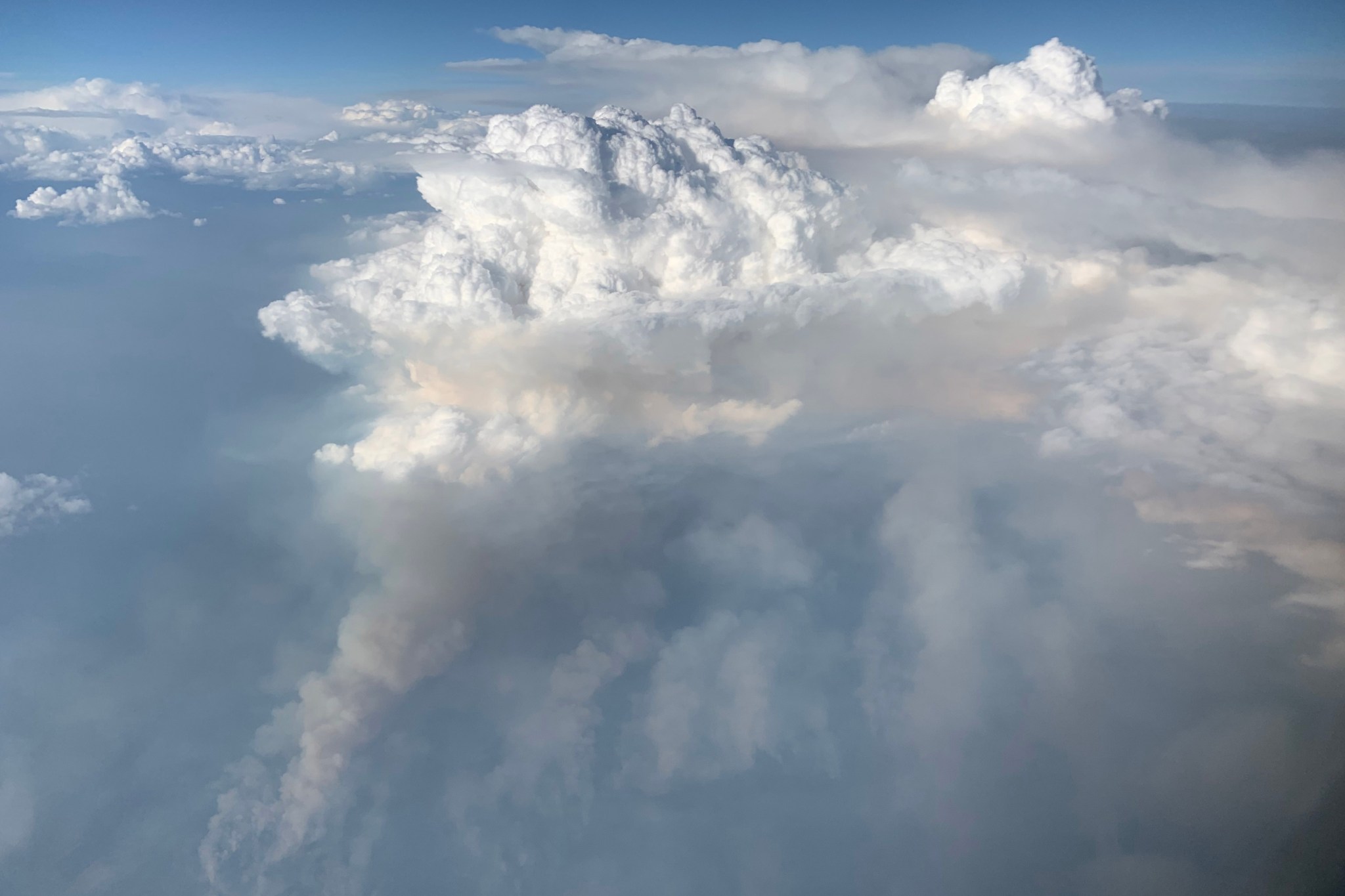
Clouds created by fire
In one of NASA's newest Earth Ventures missions, researchers will investigate the conditions that lead to the formation of pyrocumulonimbus "fire clouds." Extreme wildland fires can create their own weather and inject smoke into the stratosphere.
Courtesy of David Peterson, U.S. Naval Research Laboratory
In PYREX-the Pyrocumulonimbus Experiment-David Peterson of the Naval Research Laboratory in Washington will lead a study of pyrocumulonimbus clouds, which form when wildfires burn hot enough to make their own weather. Flying over the western U.S. and Canada, researchers will examine the fire characteristics that produce pyrocumulonimbus, while exploring the mechanisms that lead these clouds to inject smoke into the stratosphere, where it can have climate effects.
Urban air pollution
James Crawford of NASA's Langley Research Center in Hampton, Virginia, will lead HAMAQ (Hemispheric Airborne Measurements of Air Quality), a project that capitalizes on the recent launches of NASA's TEMPO pollution-monitoring satellite instrument and comparable measurements made by Korean and European satellites. Over Mexico City and a U.S. city to be determined, scientists will investigate areas of poor air quality and test how satellite information can help improve ground-based forecasting and mitigation strategies.
Shifting weather, shifting lands
Climate change is leading to more extreme droughts and rainfall events that affect the stability of hillslopes and the soil and rock on them. Led by Alexander Handwerger of NASA's Jet Propulsion Laboratory in Pasadena, California, LACCE (Landslide Climate Change Experiment) will combine airborne measurements with land-based sensors to track the way slopes and landslides are changing as water moves differently across the landscape.
Glacier retreat
John Holt of the University of Arizona will lead Snow4Flow, a project to quantify the retreat of glaciers and ice sheets in ways that can lead to better projections of land-ice change. In Alaska, southeastern Greenland, the Canadian Arctic, and Svalbard, the team will use microwave and high-frequency radar sounders to measure snow accumulation, ice melting, and changes in ice thickness and motion.
Agricultural emissions
While the burning of fossil fuels remains the leading source of carbon in our atmosphere, farmlands and ranchlands are also substantial sources of gas and particle emissions. In the NTERFAACE (Nitrogen and Carbon Terrestrial Fluxes: Agriculture, Atmospheric Composition, and Ecosystems) mission, led by Glenn Wolfe of NASA's Goddard Space Flight Center in Greenbelt, Maryland, researchers will measure the amount of greenhouse gases, nitrogen, and other pollutants that are emitted from agricultural lands across the United States.
The PYREX and Snow4Flow missions are funded at $30 million each, while the other four projects will each receive $15 million. These six investigations were selected from 42 proposals. The 2024 selections represent the fourth series of NASA Earth Venture investigations, which were first recommended by the National Research Council in 2007.
For more on NASA Earth Science, visit:
science.nasa.gov/earth
This image from the NASA/ESA Hubble Space Telescope features the barred spiral galaxy NGC 3783.
ESA/Hubble & NASA, M. C. Bentz, D. J. V. Rosario
This image from the NASA/ESA
Hubble Space Telescope
features NGC 3783, a bright barred spiral galaxy about 130 million light-years from Earth that also lends its name to the eponymous NGC 3783 galaxy group. Like galaxy clusters, galaxy groups are aggregates of gravitationally bound galaxies. Galaxy groups, however, are less massive and contain fewer members than galaxy clusters do: whereas galaxy clusters can contain hundreds or even thousands of constituent galaxies, galaxy groups do not typically include more than 50. The Milky Way is actually part of a galaxy group, known as the Local Group, which also holds two other large galaxies (Andromeda and the Triangulum galaxy), as well as several dozen satellite and dwarf galaxies. The NGC 3783 galaxy group contains 47 galaxies. It also seems to be at a fairly early stage of its evolution, making it an interesting object to study.
While the focus of this image is the spiral galaxy NGC 3783, the eye is equally drawn to the very bright object in the lower right part of this image. This is the star HD 101274. The perspective in this image makes the star and the galaxy look like close companions, but this is an illusion. HD 101274 lies only about 1,530 light-years from Earth, it is about 85,000 times closer than NGC 3783. This explains how a single star can appear to outshine an entire galaxy!
NGC 3783 is a type-1 Seyfert galaxy, which is a galaxy with a bright central region. Hubble captures it in incredible detail, from its glowing central bar to its narrow, winding arms and the dust threaded through them, thanks to five separate images taken in different wavelengths of light. In fact, the galactic center is so bright that it exhibits diffraction spikes, normally only seen on stars such as HD 101274.
Text credit: European Space Agency (ESA)
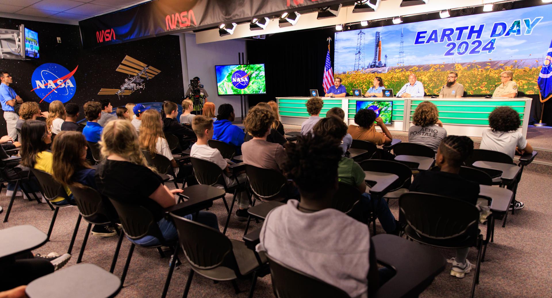
Students from Andrew Jackson Middle School in Titusville, Florida, participate in an environmentally focused Earth Day briefing on Tuesday, April 2, 2024, inside the news auditorium at the agency's Kennedy Space Center in Florida. The panelists from left to right are Messod Bendayan, NASA Communications; Kelly McCarthy, NASA's Office of STEM Engagement, Bob Kline, Kennedy's Environmental Assurance Branch; Spencer Davis, Kennedy's Exploration Ground Systems; Kim King-Wrenn, Merritt Island National Wildlife Refuge.
NASA/Kim Shiflett
At NASA's Kennedy Space Center,
sustainability
and preservation efforts here on Earth are as much of a priority as rocket launches, spacecraft, and the exploration of worlds beyond our own.
In celebration of Earth Day 2024, nearly 100 students from Andrew Jackson Middle School in Titusville, Florida, and a virtual audience of students across the country, attended NASA's Next Gen STEM Earth Day panel at the NASA News Center's John Holliman Auditorium and press site "bullpen."
On hand were NASA environmental and educational experts who discussed Kennedy's unique role balancing space launch technology and protected habitat, the center's new electric vehicle charging stations, and NASA's Earthrise educational initiative that aims to increase science, technology, engineering, and mathematics literacy.
Bob Kline, acting chief of Kennedy's Environmental Assurance Branch, helped students learn about the importance of protecting the habitat that is refuge to more than 1,500 species of plants and animals. NASA Kennedy shares a boundary with the Merritt Island National Wildlife Refuge and the Canaveral National Seashore, which encompass over 140,000 acres of land, waters, and protected habitats.
"Because we're a wildlife refuge, it's easy to think the launches would impact the wildlife, but it's mostly the buildings that might get impacted by wildlife trying to live on them," said Kline. "During renovations we've had to do special things to protect bats and other birds who live in roofs or under bridges. Everything we do, we're very mindful of the animals, whether they're endangered or not. We care about them deeply."
Panelist Kim King-Wrenn, a park ranger from Merritt Island National Wildlife Refuge, echoed Kline's message. She told students that the spaceport is one of the most biologically diverse places in the world.
Home to everything from the Florida scrub jay to endangered green sea turtles, King-Wrenn classifies Kennedy as the goldilocks of climate zones.
"Right here is where the northern temperate zone and the southern, subtropical zones come together," King-Wrenn said. "The more habitat diversity there is, the more diverse homes there are for more kinds of animals."
Students like 7th grader Zoe Oderman were fascinated by the coexistence of nature and technology across the spaceport. "The Vehicle Assembly Building was awesome, but I love that the beaches at Kennedy Space Center give turtles a place to lay their eggs, because other places in the area don't," Oderman said.
Kennedy employee Spencer Davis discussed the installation of 56 electric vehicle charging stations during his time at the NASA Transportation Office on center. The new infrastructure helps support a fleet of electric government vehicles including the all-electric crew transport vehicles that will take Artemis astronauts from their crew quarters to the launch pad.
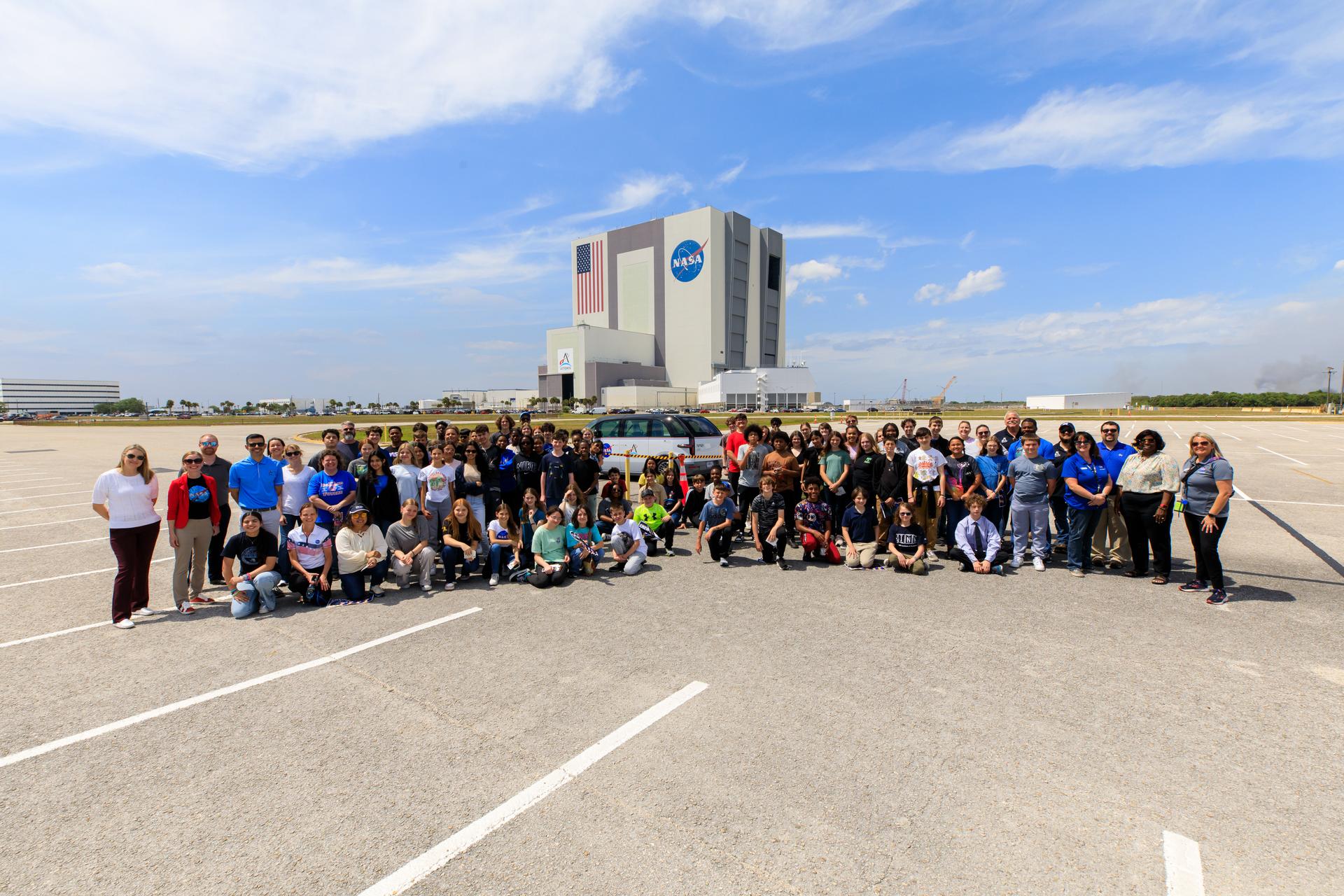
Students from Andrew Jackson Middle School in Titusville, Florida, pose for a photo with one of the Artemis crew transportation vehicles in front of the Vehicle Assembly Building at NASA's Kennedy Space Center in Florida on Tuesday, April 2, 2024. As part of NASA's NextGen STEM project, the students joined others from across the country who participated virtually for an environmentally focused Earth Day briefing held inside Kennedy's news auditorium to discuss how technology and science coexist with nature at the spaceport.
NASA/Kim Shiflett
Later this summer, Davis and his team will be honored at the White House for these efforts to facilitate a future of zero carbon emission government vehicles and help save taxpayer money.
"The big takeaway here is in order to charge up and drive one of Kennedy's Chevrolet Bolts 100 miles, it only costs $2.80," Davis said. "That's basically the price of a soft drink."
The students also learned about
Earthrise
from panelist Kelly McCarthy, program specialist with NASA's Office of STEM Engagement at the agency's Stennis Space Center in Mississippi.
The NASA education initiative provides educators with access to monthly collections of resources aimed at increasing STEM literacy and understanding the importance of protecting our home planet.
"Earthrise is a really good way to find out the most relevant and useful solutions-based resources that exist right now," McCarthy said.
Besides offering their expertise on sustainable practices as well as words of encouragement to the future stewards of our planet, the panelists inspired students to pursue STEM careers, including at Kennedy.
"You can do anything you want to do out here, and if you really apply yourself you can get into any field," Davis told the students. "Don't be afraid to step outside the box. Don't be afraid to do something completely different, even if it's scary. Take every opportunity and seize the moment."
The event was coordinated through the Next Gen STEM project in NASA's
Office of STEM Engagement
, which reaches students in schools and informal classrooms across the county.
View NASA's Next Gen STEM Earth Day Student Briefing here:
AI for Earth: How NASA's Artificial Intelligence and Open Science Efforts Combat Climate Change
Lights brighten the night sky in this image of Europe, including Poland, taken from the International Space Station.
NASA
As extreme weather events increase around the world due to climate change, the need for further research into our warming planet has increased as well. For NASA, climate research involves not only conducting studies of these events, but also empowering outside researchers to do the same. The artificial intelligence (AI) efforts spearheaded by the agency offer a powerful tool to accomplish these goals.
In 2023, NASA teamed up with IBM Research to create an AI geospatial foundation model. Trained on vast amounts of NASA's widely used
Harmonized Landsat and Sentinel-2 (HLS)
data, the model provides a base for a variety of AI-powered studies to tackle environmental challenges. In keeping with open science principles,
the model is freely available for anyone to access
.
Foundation models serve as a baseline from which scientists can develop a diverse set of applications, enabling powerful and efficient solutions. "Foundation models only know what things are represented in the data," explained Manil Maskey, the data science lead at NASA's Office of the Chief Science Data Officer (OCSDO). "It's like a Swiss Army Knife-it can be used for multiple different things."
Once a foundation model is created, it can be trained on a small amount of data to perform a specific task. To date, the Interagency Implementation and Advanced Concept Team (IMPACT) along with collaborators have demonstrated the geospatial foundation model's capabilities by fine-tuning it to detect burn scars, to delineate flood water, and to classify crop and other land use categories.
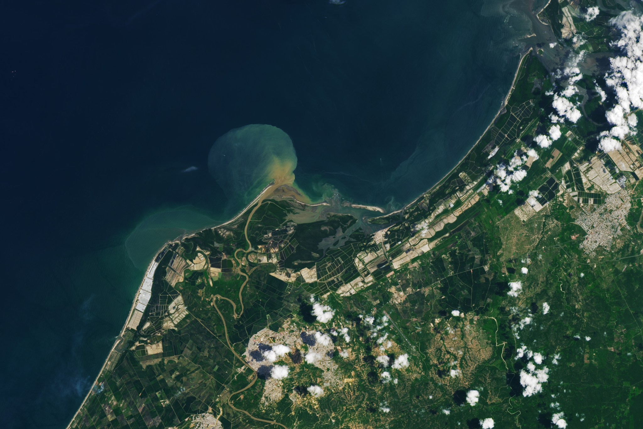
Rectangular ponds for shrimp farming line the coast of northern Peru in this image captured on March 14, 2024 by the OLI-2 (Operational Land Imager-2) on Landsat 9.
NASA Earth Observatory / Lauren Dauphin
Because of the computational resources required to create the initial foundation model, a partnership was necessary for success. In this case, NASA brought the data and scientific knowledge, while IBM brought the computing power and AI algorithm optimization expertise. The team's shared commitment to making their research accessible through open science principles ensures that their model can be useful to as many researchers as possible.
"To build a foundation model at scale, we realized early on that it's not feasible for one institution to build it," Maskey said. "Everything we have done on our foundation models has been open to the public, all the way from pre-training data, code, best practices, model weights, fine-tuning training data, and publications. There's transparency, so researchers can trace why certain things were used in terms of data or model architecture."
Following on from the success of their geospatial foundation model, NASA and IBM Research are continuing their partnership to create a new, similar model for weather and climate studies. They are collaborating with Oak Ridge National Laboratory (ORNL), NVIDIA, and several universities to bring this model to life.
This time, the main dataset will be the
Modern-Era Retrospective analysis for Research and Applications, Version 2 (MERRA-2)
, a huge collection of atmospheric reanalysis data that spans from 1980 to the present day. Like the geospatial foundation model, the weather and climate model is being developed with an open science approach, and will be available to the public in the near future.
Covering all aspects of Earth science would take several foundation models trained on different types of datasets. However, Maskey believes those future models might someday be combined into one comprehensive model, leading to a "digital twin" of the Earth that would provide unparalleled analysis and predictions for all kinds of climate and environmental events.
Whatever innovations the future holds, NASA and IBM's geospatial and climate foundation models will enable leaps in Earth science like never before. Though powerful AI tools will enhance researchers' work, the team's dedication to open science supercharges the possibilities for discovery by allowing anyone to put those tools into practice and pave the way for groundbreaking research to help better care for the planet.
For more information about open science at NASA, visit:
https://science.nasa.gov/open-science/
By
Lauren Leese
Web Content Strategist for the Office of the Chief Science Data Officer
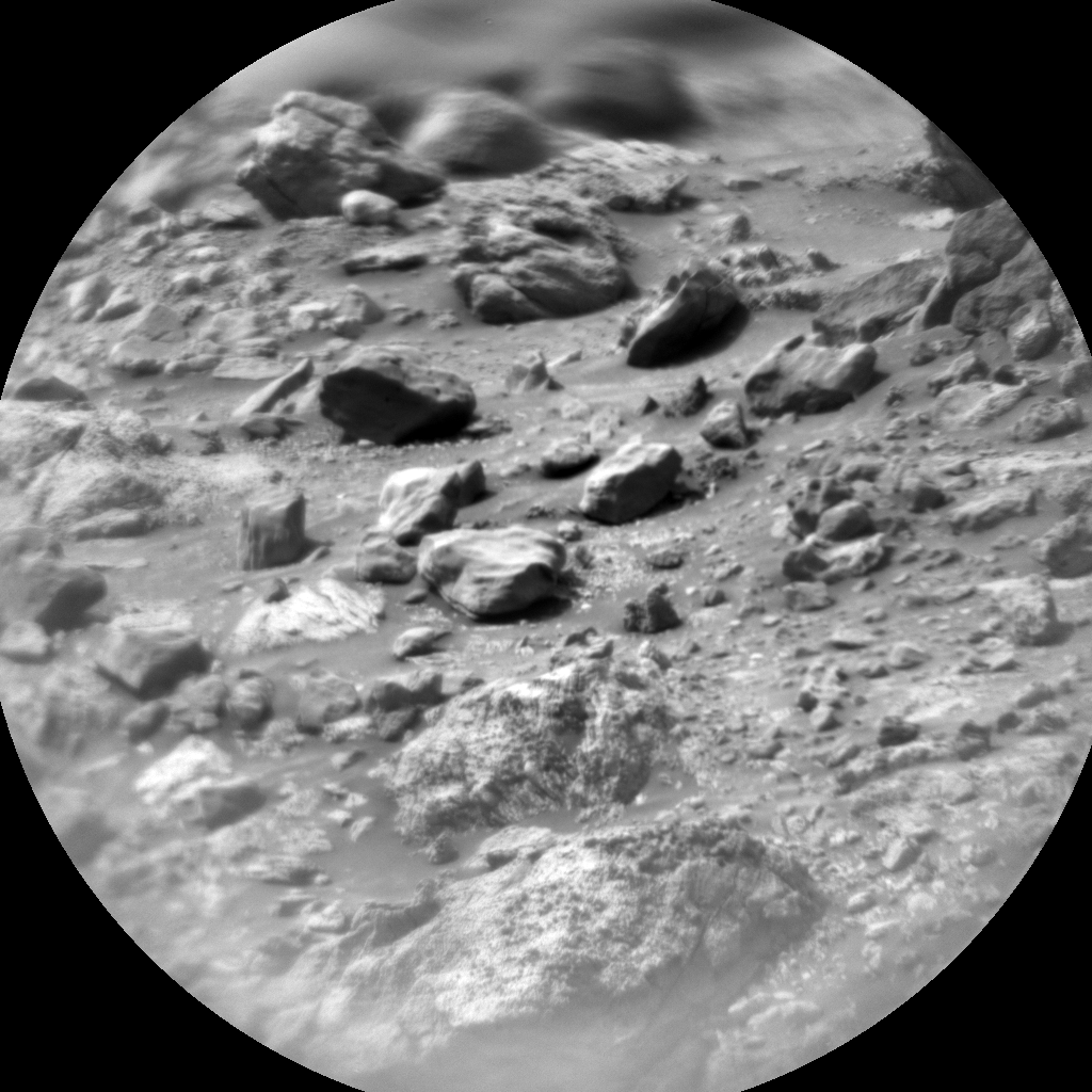
This image was taken by Chemistry & Camera (ChemCam) onboard NASA's Mars rover Curiosity on Sol 4158 (2024-04-17 07:52:27 UTC).
NASA/JPL-Caltech/LANL
Earth planning date: Wednesday, April 17, 2024
Curiosity continues to make progress along the margin of upper Gediz Vallis ridge, investigating the broken bedrock in our workspace and acquiring images of the ridge deposit as the rover drives south.
Today's 2-sol plan focused on a DRT, contact science, and drive on the first sol, followed by untargeted remote sensing on the second sol. The team had to make some decisions at the start of planning about whether to drive on the first or second sol of this plan, and how that would affect the upcoming weekend activities. As it turned out, the team was able to fit all of the desired contact science and remote sensing activities on the first sol, in addition to the drive on the first sol, which means we'll be able to downlink more information about our end-of-drive location to better inform planning for the weekend. Weekend plans provide opportunities for a lot of great contact science, so it will be really helpful to have that additional data down for planning.
That means the first sol of this plan is fully loaded! The plan begins with a DRT activity to expose a fresh surface on the bedrock target "Tilden Lake," followed by APXS integrations to investigate its composition. Then the Geology theme group planned several hours of remote sensing activities, including ChemCam LIBS on the bedrock target "Curry Village," which has a similar "dragon scale" texture (or "tire tracks") to what we had observed in the previous workspace. This big remote sensing block also includes ChemCam long distance RMI mosaics to assess the stratigraphy at Gediz Vallis ridge and the distant butte Kukenan. These long distance RMI images reveal a lot of great detail about distant targets, like the diversity of clasts at Gediz Vallis ridge, as seen in the above image.
The plan also includes a number of Mastcam activities to characterize local textures, sedimentary structures, dark rocks, and sandy aeolian bedforms (known as Transverse Aeolian Ridges, aka TARs) in a nearby trough. The Environmental theme group also planned activities to monitor the movement of fines on the rover deck, search for dust devils, and monitor atmospheric dust. After this big remote sensing block, Curiosity will use MAHLI to image the contact science target, and then continue driving south. The second sol includes untargeted activities like an autonomously selected ChemCam AEGIS target, additional Navcam deck monitoring, and Navcam line-of-sight observations. After the drive we'll take post drive imaging to prepare for the next plan.
Looking forward to seeing what other surprises our next workspace will reveal!
Written by Lauren Edgar, Planetary Geologist at USGS Astrogeology Science Center
The ocean holds about 97 percent of Earth’s water and covers 70 percent of our planet’s surface. According to the United Nations, the ocean may be home to 50 to 80 percent of all life on Earth. Even if you live hundreds of miles from a coast, what happens in the ocean is fundamental to your life.